机器学习
KNN(k-nearest neighbor),即K近邻算法。当需要表示一个样本(值)的时候,就使用与该样本最接近的K个邻居来决定。KNN既可以用于分类,也可以用于回归
KNN算法的过程为:
·从训练集中选择离待预测样本最近的k个样本。
·根据这k个样本计算待预测样本的值(属于哪个类别或者一个具体数值)
欧氏距离
根据以上定义,欧氏距离可以写为:
\(d_{xy}=\sqrt{\sum_{k=1}^{n}(x_k-y_k)^2}\)
数据集的划分
训练数据:用于训练,构建模型
测试数据:在模型检验时使用,用于评估模型是否有效
测试集20%~30%
训练集特征值,测试集特征值,训练集目标值,测试集目标值
x_train, x_test, y_train, y_test
import numpy as np
import pandas as pd
#读取鸢尾花数据集,header参数制定标题的行。,默认为0,没有标题用None。
data = pd.read_csv(r"./dataset/iris.arff.csv", header=0)

# data.head(10)# 默认前5行
# data.tail() # 默认末尾5行
data.sample(10) # 默认随即抽取1条
# 将类别文本映射成为数值类型,class为列名,后面列名重命名
data["class"]=data["class"].map({"Iris-versicolor":0,"Iris-setosa":1, "Iris-virginica":2})
# 删除 sepallength名字一列
data.drop("sepallength", axis=1,inplace=True)
# 查看是否重复记录
# data.duplicated().any()
# 查看重复记录
# len(data)
# 删除重复记录
data.drop_duplicates(inplace=True)
# 查看各个类别多少记录
data["class"].value_counts()
class KNN:
    """使用python语言实现k近邻算法。(实现分类)"""
    def __init__(self, k):
        """初始化方法
        Parameters
        -------
        k:int
        邻居的个数
        """
        self.k=k

    def fit(self, X, y):
        """
        训练方法
        Parameters
        ————————
        X:类数组类型, 形状为:[样本数量,特征数量]
        待训练的样本特征(属性)
        y:类数组类型样本的数量:[样本数量]
        每个样本的目标值(标签)
        """
        # 将x转化为array数组类型
        self.X = np.asarray(X)
        self.y = np.asarray(y)

    def predict(self, X):
        """
        根据参数传递的样本,对样本进行预测
        Parameters
        -----
        X:类数组类型, 形状为:[样本数量,特征数量]
        待训练的样本特征(属性)
        Parameters
        -----
        result:数组类型
        预测的结果。
        """
        X = np.asarray(X)
        result = []
        for x in X:
            # 对于测试集中的每一个样本,依次与训练集中的所有样本求距离, axis=1表示每一行相加
            dis = np.sqrt(np.sum((x - self.X) ** 2, axis=1))
            # 返回数组排序后,每个元素在原数组(排序前的数组)中的索引
            index = dis.argsort()
            # 进行截断,之区前k个元素,[取距离最近的k个元素索引]
            index = index[:self.k]
            # 返回数组中每个元素出现的次数,元素必须是非负整数
            count = np.bincount(self.y[index])
            # 返回ndarray数组中,值最大的元素对应的索引,该索引就是我们判定的类别
            # 最大元素索引,就是出现次数最多的元素.
            result.append(count.argmax())
        return np.asarray(result)

    def predict2(self, X):
        """
        根据参数传递的样本,对样本进行预测(考虑权重,是哟个距离的倒数作为权重)
        Parameters
        -----
        X:类数组类型, 形状为:[样本数量,特征数量]
        待训练的样本特征(属性)
        Parameters
        -----
        result:数组类型
        预测的结果。
        """
        X = np.asarray(X)
        result = []
        for x in X:
            # 对于测试集中的每一个样本,依次与训练集中的所有样本求距离, axis=1表示每一行相加
            dis = np.sqrt(np.sum((x - self.X) ** 2, axis=1))
            # 返回数组排序后,每个元素在原数组(排序前的数组)中的索引
            index = dis.argsort()
            # 进行截断,之区前k个元素,[取距离最近的k个元素索引]
            index = index[:self.k]
            # 返回数组中每个元素出现的次数,元素必须是非负整数[使用weight考虑权重,权重为距离的倒数]
            count = np.bincount(self.y[index], weights=1 / dis[index])
            # 返回ndarray数组中,值最大的元素对应的索引,该索引就是我们判定的类别
            # 最大元素索引,就是出现次数最多的元素.
            result.append(count.argmax())
        return np.asarray(result)
# 提取每个类数据
t0 = data[data["class"] == 0]
t1 = data[data["class"] == 1]
t2 = data[data["class"] == 2]
# 对每个类别数据进行洗牌,  这里的random_state就是为了保证程序每次运行都分割一样的训练集和测试集
t0 = t0.sample(len(t0), random_state=0)
t1 = t1.sample(len(t1), random_state=0)
t2 = t2.sample(len(t2), random_state=0)
# 构建训练集与测试集
train_X = pd.concat([t0.iloc[:40,:-1],t1.iloc[:40,:-1],t2.iloc[:40,:-1]],axis=0)
train_y = pd.concat([t0.iloc[:40,-1],t1.iloc[:40,-1],t2.iloc[:40,-1]],axis=0)
test_X = pd.concat([t0.iloc[40:,:-1],t1.iloc[40:,:-1],t2.iloc[40:,:-1]],axis=0)
test_y = pd.concat([t0.iloc[40:,-1],t1.iloc[40:,-1],t2.iloc[40:,-1]],axis=0)
# 创建KNN对象,进行训练与测试
knn = KNN(k=3)
#进行训练
knn.fit(train_X, train_y)
# 进行测试.获取测试的结果
result = knn.predict(test_X)
# display(result)
# display(test_y)
display(np.sum(result == test_y))
display(np.sum(result == test_y)/len(result))
"""
21
0.9545454545454546
"""
# 考虑权重
result2 = knn.predict2(test_X)
display(np.sum(result2 == test_y))
"""21"""
import matplotlib as mpl
import matplotlib.pyplot as plt
import matplotlib.font_manager as fm
# 默认情况下,matplot不支持中文显示,我们需要进行一下设置
# 设置字体为ie黑体,以支持中文显示
font = fm.FontProperties(fname='/home/yys/.local/lib/python3.8/site-packages/matplotlib/mpl-data/fonts/ttf/msyh.ttf')
# 设置在中文字体时,能够正常显示负号(-)
mpl.rcParams['axes.unicode_minus'] = False
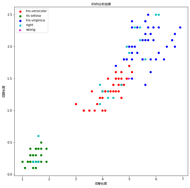
# {"Iris-versicolor":0,"Iris-setosa":1, "Iris-virginica":2}
# 设置画布大小
plt.figure(figsize=(10,10))
# 绘制训练集数据
plt.scatter(x=t0["petallength"][:40], y=t0["petalwidth"][:40], color="r", label="Iris-versicolor")
plt.scatter(x=t1["petallength"][:40], y=t1["petalwidth"][:40], color="g", label="ris-setosa")
plt.scatter(x=t2["petallength"][:40], y=t2["petalwidth"][:40], color="b", label="Iris-virginica")
# 绘制测试集数据
right = test_X[result == test_y]
wrong = test_X[result != test_y]
plt.scatter(x=right["petallength"], y=right["petalwidth"], color="c",marker="X" , label="right")
plt.scatter(x=wrong["petallength"], y=wrong["petalwidth"], color="m",marker=">" , label="wrong")
plt.xlabel("花萼长度" , fontproperties=font)
plt.ylabel("花瓣长度",fontproperties=font)
plt.title("KNN分析结果",fontproperties=font)
plt.legend(loc="best")
plt.show()
Python - Ubuntu环境 matplotlib 中文显示问题
Ubuntu系统上使用python 的 matplotlib库展示和中文相关的信息时,往往无法显示,出现乱码.
原因是,缺乏对中文字体库的支持.
1. 解决方案
两种中文字体(Ubuntu):
[1] - 微软雅黑字体msyh.ttf:http://siwei.me/system/resources/W1siZiIsIjIwMTYvMDcvMTIvMDdfNTdfMjNfMTM5X21zeWgudHRmIl1d/msyh.ttf
[2] - 黑体 SimHei字体:http://fontzone.net/download/simhei
使用方法:
[1] - 查看 matplotlib 字体的安装位置:
locate -b '\mpl-data'
一般路径,如:/home/yys/.local/lib/python3.8/site-packages/matplotlib/mpl-data/fonts/ttf/
[2] - 把下载的字体放到该目录下:
sudo mv msyh.ttf /home/yys/.local/lib/python3.8/site-packages/matplotlib/mpl-data/fonts/ttf/
或
sudo mv simhei.ttf /home/yys/.local/lib/python3.8/site-packages/matplotlib/mpl-data/fonts/ttf/
[3] - 删除当前用户 matplotlib 的缓冲文件.
cd ~/.cache/matplotlib
rm -rf *.*
注:matplotlib缓存文件一般在~/.cache/matplotlib. 也可以查看缓冲文件位置:
import matplotlib
print(matplotlib.get_cachedir())
[4] - matplotlib 使用指定字体:
import matplotlib.pyplot as plt

plt.rcParams[u'font.sans-serif'] = ['SimHei']
#或
plt.rcParams['font.family'] = ['Microsoft YaHei']
plt.rcParams['axes.unicode_minus'] = False
或者:
import matplotlib as mpl
import matplotlib.pyplot as plt
import matplotlib.font_manager as fm
# 默认情况下,matplot不支持中文显示,我们需要进行一下设置
# 设置字体为ie黑体,以支持中文显示
font = fm.FontProperties(fname='/home/yys/.local/lib/python3.8/site-packages/matplotlib/mpl-data/fonts/ttf/msyh.ttf')
# 设置在中文字体时,能够正常显示负号(-)
mpl.rcParams['axes.unicode_minus'] = False
# {"Iris-versicolor":0,"Iris-setosa":1, "Iris-virginica":2}
# 设置画布大小
plt.figure(figsize=(10,10))
# 绘制训练集数据
plt.scatter(x=t0["petallength"][:40], y=t0["petalwidth"][:40], color="r", label="Iris-versicolor")
plt.scatter(x=t1["petallength"][:40], y=t1["petalwidth"][:40], color="g", label="ris-setosa")
plt.scatter(x=t2["petallength"][:40], y=t2["petalwidth"][:40], color="b", label="Iris-virginica")
# 绘制测试集数据
right = test_X[result == test_y]
wrong = test_X[result != test_y]
plt.scatter(x=right["petallength"], y=right["petalwidth"], color="c",marker="X" , label="right")
plt.scatter(x=wrong["petallength"], y=wrong["petalwidth"], color="m",marker=">" , label="wrong")
plt.xlabel("花萼长度" , fontproperties=font)
plt.ylabel("花瓣长度",fontproperties=font)
plt.title("KNN分析结果",fontproperties=font)
plt.legend(loc="best")
plt.show()
import numpy as np
import pandas as pd
data = pd.read_csv(r"./dataset/iris.csv")
# 删除不需要的内容class(特征),因为现在进行回归预测,类别信息就没有用处了
data.drop(["Species"], axis=1, inplace=True)
# 删除重复记录
data.drop_duplicates(inplace=True)
"""
Unnamed: 0 Sepal.Length Sepal.Width Petal.Length Petal.Width
0 1 5.1 3.5 1.4 0.2
1 2 4.9 3.0 1.4 0.2
2 3 4.7 3.2 1.3 0.2
3 4 4.6 3.1 1.5 0.2
4 5 5.0 3.6 1.4 0.2
... ... ... ... ... ...
145 146 6.7 3.0 5.2 2.3
146 147 6.3 2.5 5.0 1.9
147 148 6.5 3.0 5.2 2.0
148 149 6.2 3.4 5.4 2.3
149 150 5.9 3.0 5.1 1.8
150 rows × 5 columns
"""
class KNN:
    """使用Python实现k近邻算法.(回归预测)
    该算法用于回归预测,根据前3个特征值,寻找最近的k个邻居,然后根据k个邻居的第4个特征属性,
    去预测当前样本的4个特征值
    """

    def __init__(self, k):
        """
        初始化方法
        Parameters
        -------
        k:int
            邻居个数
        """
        self.k = k

    def fit(self, X, y):
        """训练方法
        Parameters
        ----------
        X:类数组类型(特征矩阵).形状为[样本数量,特征数量]
          待训练的样本特征(属性)
        y:类数组类型(目标标签).形状为[样本数量]
          每个样本的目标值[标签]
        """
        self.X = np.asarray(X)
        self.y = np.asarray(y)

    def predict(self, X):
        """
        根据参数传递参数,对样本进行预测.
        Paramters:
        --------
        X:类数组类型(特征矩阵).形状为[样本数量,特征数量]
          待训练的样本特征(属性)

        Return
        -------
        result : 数组类型
        ---预测的结果值
        """
        # 转换为数组类型
        X = np.asarray(X)
        # 保存预测结果值
        result = []
        for x in X:
            # 计算距离.(计算与训练集中那个x的距离)
            dis = np.sqrt(np.sum((x-self.X)**2, axis=1))
            # 返回数组排序后,每个元素在原数组中(排序之前的数组)的索引
            index = dis.argsort()
            # 取前k个距离最近的索引(在原数组中的索引)
            index = index[:self.k]
            # 计算均值,然后加入到结果列表中
            result.append(np.mean(self.y[index]))
        return np.array(result)


    def predict2(self, X):
        """
        根据参数传递参数,对样本进行预测.
        权重的计算方式:使用每个节点(邻居)距离的倒数/所有节点距离之和
        Paramters:
        --------
        X:类数组类型(特征矩阵).形状为[样本数量,特征数量]
          待训练的样本特征(属性)

        Return
        -------
        result : 数组类型
        ---预测的结果值
        """
        # 转换为数组类型
        X = np.asarray(X)
        # 保存预测结果值
        result = []
        for x in X:
            # 计算距离.(计算与训练集中那个x的距离)
            dis = np.sqrt(np.sum((x-self.X)**2, axis=1))
            # 返回数组排序后,每个元素在原数组中(排序之前的数组)的索引
            index = dis.argsort()
            # 取前k个距离最近的索引(在原数组中的索引)
            index = index[:self.k]
            # 求所有邻居节点的倒数之和.[注意,最后加上一个很小的值,为了避免除数(距离)为0的情况]
            s = np.sum(1 / (dis[index]+0.001))
            # 使用邻居节点距离的倒数,除以倒数之和,得到权重
            weight = (1 / (dis[index]) + 0.001) / s
            # 使用邻居结点标签值,乘以对应的权重,然后相加,得到最终预测的预测结果
            result.append(np.sum(self.y[index] * weight))
        return np.array(result)
# random_state=0可以重现随机序列
t = data.sample(len(data), random_state=0)
train_X = t.iloc[:120, :-1]
train_y = t.iloc[:120, -1]
test_X = t.iloc[120:, :-1]
test_y = t.iloc[120:, -1]
knn = KNN(k=3)
knn.fit(train_X, train_y)
result = knn.predict(test_X)
display(result)
np.mean(np.sum((result - test_y)**2))
display(test_y.values)
"""
array([0.3 , 2.06666667, 0.26666667, 0.2 , 1.93333333,
0.63333333, 1.83333333, 1.43333333, 1.4 , 1.33333333,
2.06666667, 2.13333333, 1.26666667, 1.43333333, 0.36666667,
1.4 , 2.06666667, 2.36666667, 0.2 , 1.33333333,
1.33333333, 1.3 , 1.46666667, 0.16666667, 0.3 ,
0.2 , 2.06666667, 1.36666667, 2.13333333, 0.23333333])
array([0.2, 2. , 0.3, 0.2, 1.9, 0.2, 2.4, 1.3, 1.2, 1. , 2.3, 2.3, 1.5,
1.7, 0.2, 1. , 2.4, 1.9, 0.2, 1.3, 1.3, 1.8, 1.3, 0.2, 0.4, 0.1,
1.8, 1. , 2.2, 0.2])
"""
result = knn.predict2(test_X)
display(np.mean(np.sum((result-test_y)**2)))
"""
1.717401375837938
"""
import matplotlib as mpl
import matplotlib.pyplot as plt
import matplotlib.font_manager as fm
# 设置字体为ie黑体,以支持中文显示
font = fm.FontProperties(fname='/home/yys/.local/lib/python3.8/site-packages/matplotlib/mpl-data/fonts/ttf/msyh.ttf')
# 设置在中文字体时,能够正常显示负号(-)
mpl.rcParams['axes.unicode_minus'] = False
plt.figure(figsize=(10, 10))
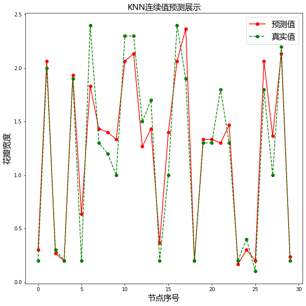
# 绘制预测值
plt.plot(result, 'ro-', label= "预测值")
# 绘制真真实值
plt.plot(test_y.values, "go--", label= "真实值")
plt.title("KNN连续值预测展示", fontproperties=font)
plt.xlabel("节点序号", fontproperties=font)
plt.ylabel("花瓣宽度", fontproperties=font)
# 添加prop=font为了label中文不乱吗
plt.legend(prop=font, loc="best")
plt.show()
线性回归,就是用一条直线来解释自变量与因变量之间的关系。我们可以将线性回归表示为:
\(y=w^0+w^1x^1+w^2x^2+...+w^n+x^n=\sum_{i=0}^{n}w^ix^i=W^TX\)
线性回归目标函数为:
\(j(w)=\frac{1}{2}\sum_{i=1}^{n}(y^{(i)}+{\hat{y} }^{(i)})^2\)
我们可以采用两种方式进行求解
·最小二乘法
·梯度下降法
import numpy as np
import pandas as pd
data = pd.read_csv(r"./dataset/boston.csv")
"""
波士顿房价数据集字段说明
crim:房屋所在镇的犯罪率
zn:面积大于25000平方英尺住宅所占的比例
indus:房屋所在镇非零售区域所占比例
chas:房屋是否位于河边,如果位于河边,则值为1,否则值为0
nox:一氧化氮的浓度
rm:平均房间数量
age:1940年前建成房屋所占的比例
dis:房屋距离波士顿五大就业中心的加权距离
rad:距房屋最近的公路
tax:财产税额度
ptratio:房屋所在镇师生比例
black:日计算公式:1000(房屋所在镇非美籍人口所在比例-0632
lstat:弱势群体人口所占比例
medv:房屋的平均价格
"""
# 查看数据的基本信息,同时,也可以用来查看,各个特征列是否存在缺失值
# data.info()
# 查看是否有重复值,False表示没有重复值
# data.duplicated().any()
# 删除不需要的内容class(特征),因为现在进行回归预测,类别信息就没有用处了
data.drop(["Unnamed: 0"], axis=1, inplace=True)
"""
crim zn indus chas nox rm age dis rad tax ptratio black lstat medv
0 0.00632 18.0 2.31 0 0.538 6.575 65.2 4.0900 1 296 15.3 396.90 4.98 24.0
1 0.02731 0.0 7.07 0 0.469 6.421 78.9 4.9671 2 242 17.8 396.90 9.14 21.6
2 0.02729 0.0 7.07 0 0.469 7.185 61.1 4.9671 2 242 17.8 392.83 4.03 34.7
3 0.03237 0.0 2.18 0 0.458 6.998 45.8 6.0622 3 222 18.7 394.63 2.94 33.4
4 0.06905 0.0 2.18 0 0.458 7.147 54.2 6.0622 3 222 18.7 396.90 5.33 36.2
... ... ... ... ... ... ... ... ... ... ... ... ... ... ...
501 0.06263 0.0 11.93 0 0.573 6.593 69.1 2.4786 1 273 21.0 391.99 9.67 22.4
502 0.04527 0.0 11.93 0 0.573 6.120 76.7 2.2875 1 273 21.0 396.90 9.08 20.6
503 0.06076 0.0 11.93 0 0.573 6.976 91.0 2.1675 1 273 21.0 396.90 5.64 23.9
504 0.10959 0.0 11.93 0 0.573 6.794 89.3 2.3889 1 273 21.0 393.45 6.48 22.0
505 0.04741 0.0 11.93 0 0.573 6.030 80.8 2.5050 1 273 21.0 396.90 7.88 11.9
506 rows × 14 columns
"""
class linearRegression:
    """使用Python实现的线性回归(最小二乘法)"""

    def fit(self, X, y):
        """根据提供的训练数据X,对模型进行训练
        Parameters
        ---------
        X:类数组类型.形状:[样本数量, 特征数量]
           特征矩阵,用来对模型进行训练
        y:类数组类型,形状:[样本数量]

        """
        # 说明:如果x是数组对象的一部分,而不是完整的对象数据(例如,X是由其他对象通过切片传递来的)
        # 则无法完成矩阵的转换
        # 这里创建X的拷贝对象,避免转换矩阵的时候失败
        X = np.asmatrix(X.copy())
        # y是一维结构(行向两或列向量), 一维结构可以不用进行拷贝.
        # 注意:我们现在要进行矩阵的运算,因此需要是二维结构,我们通过reshape方法进行转换
        y = np.asmatrix(y).reshape(-1, 1)
        # 通过最小二乘法公式.求解出最佳权重值,.T转置, .I求逆
        self.w_ = (X.T * X).I * X.T * y
    def predict(self, X):
        """根据参数传递的样本x, 对样本数据进行预测.
        Parameters
        -------
        X:类数组类型.形状:[样本数量, 特征数量]
           待预测的样本特征(属性).
        Return
        ------
        result:数组类型
            预测的结果.
        """
        # 将x转换成矩阵,需要对X进行拷贝
        X = np.asmatrix(X.copy())
        result = X * self.w_
        # 将矩阵转换成ndarray数组,进行扁平化处理,然后返回结果.
        # 使用ravel可以将数组进行扁平化处理
        return np.array(result).ravel()
# 不考虑截距
t = data.sample(len(data), random_state=0)
train_X = t.iloc[:400, :-1]
train_y = t.iloc[:400, -1]
test_X = t.iloc[400:, :-1]
test_y = t.iloc[400:, -1]
lr = linearRegression()
lr.fit(train_X, train_y)
result = lr.predict(test_X)
# result
display(np.mean((result - test_y) ** 2 ))
# 查看权重值
display(lr.w_)
16.89257506996371
matrix([[-2.25548227e-03],
[-9.36187378e-02],
[ 4.57218914e-02],
[ 3.67703558e-03],
[ 2.43746753e+00],
[-2.96521997e+00],
[ 5.61875896e+00],
[-4.94763610e-03],
[-8.73950002e-01],
[ 2.49282064e-01],
[-1.14626177e-02],
[-2.50045098e-01],
[ 1.49996195e-02],
[-4.56440342e-01]])
# 考虑截距,增加一列,该列所有值都是1.
t = data.sample(len(data), random_state=0)
# 按照习惯,截矩为w0,我们为之而配上一个x0,x0列放在最前
new_columns = t.columns.insert(0, "intercept")
# 重新安排列的顺序,如果为空,则使用fill_alue参数制定值进行填充。
t = t.reindex(columns=new_columns, fill_value=1)
train_X = t.iloc[:400, :-1]
train_y = t.iloc[:400, -1]
test_X = t.iloc[400:, :-1]
test_y = t.iloc[400:, -1]
lr = linearRegression()
lr.fit(train_X, train_y)
result = lr.predict(test_X)
# result
display(np.mean((result - test_y) ** 2 ))
# 查看权重值
display(lr.w_)
17.097531384667846
matrix([[ 4.00542166e+01],
[-1.10490198e-01],
[ 4.11074548e-02],
[ 1.14986147e-02],
[ 2.03209693e+00],
[-1.95402764e+01],
[ 3.28900304e+00],
[ 6.91671720e-03],
[-1.39738261e+00],
[ 3.78327573e-01],
[-1.54938397e-02],
[-8.64470498e-01],
[ 8.29999966e-03],
[-5.66991979e-01]])
import matplotlib as mpl
import matplotlib.pyplot as plt
import matplotlib.font_manager as fm
# 设置字体为ie黑体,以支持中文显示
font = fm.FontProperties(fname='/home/yys/.local/lib/python3.8/site-packages/matplotlib/mpl-data/fonts/ttf/msyh.ttf', size=16)
# 设置在中文字体时,能够正常显示负号(-)
mpl.rcParams['axes.unicode_minus'] = False
plt.figure(figsize=(10,10))
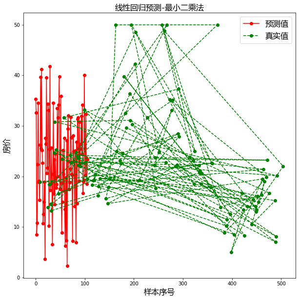
# 绘制预测值
plt.plot(result, "ro-", label="预测值")
# 绘制真实值
plt.plot(test_y, "go--", label="真实值")
plt.title("线性回归预测-最小二乘法", fontproperties=font)
plt.xlabel("样本序号", fontproperties=font)
plt.ylabel("房价", fontproperties=font)
plt.legend(prop=font, loc="best")
plt.show()
import numpy as np
import pandas as pd
data = pd.read_csv(r"./dataset/boston.csv")
data.drop(["Unnamed: 0"], axis=1, inplace=True)
crim zn indus chas nox rm age dis rad tax ptratio black lstat medv
0 0.00632 18.0 2.31 0 0.538 6.575 65.2 4.0900 1 296 15.3 396.90 4.98 24.0
1 0.02731 0.0 7.07 0 0.469 6.421 78.9 4.9671 2 242 17.8 396.90 9.14 21.6
2 0.02729 0.0 7.07 0 0.469 7.185 61.1 4.9671 2 242 17.8 392.83 4.03 34.7
3 0.03237 0.0 2.18 0 0.458 6.998 45.8 6.0622 3 222 18.7 394.63 2.94 33.4
4 0.06905 0.0 2.18 0 0.458 7.147 54.2 6.0622 3 222 18.7 396.90 5.33 36.2
... ... ... ... ... ... ... ... ... ... ... ... ... ... ...
501 0.06263 0.0 11.93 0 0.573 6.593 69.1 2.4786 1 273 21.0 391.99 9.67 22.4
502 0.04527 0.0 11.93 0 0.573 6.120 76.7 2.2875 1 273 21.0 396.90 9.08 20.6
503 0.06076 0.0 11.93 0 0.573 6.976 91.0 2.1675 1 273 21.0 396.90 5.64 23.9
504 0.10959 0.0 11.93 0 0.573 6.794 89.3 2.3889 1 273 21.0 393.45 6.48 22.0
505 0.04741 0.0 11.93 0 0.573 6.030 80.8 2.5050 1 273 21.0 396.90 7.88 11.9
506 rows × 14 columns
class LinearRegression:
    """使用Python语言实现线性回归算法.(剃度下降)"""

    def __init__(self,alpha, times):
        """初始化方法.
        Parameters
        ------
        alpha: float
          学习率.用来控制步长.(权重调整幅度)
          times:int
          循环迭代次数
        """
        self.alpha = alpha
        self.times = times
    def fit(self, X, y):
        """根据提供训练数据,对模型训练
        Parameters
        -----
        X : 类数组类型.形状:[样本数量,特征数量]
            待训练的样本特征属性.[特征矩阵]
        y : 类数组类型.形炸ung:[样本数量]
            目标值(标签信息).
        """
        X = np.asarray(X)
        y = np.asarray(y)
        # 创建权重的向量,初始值为0(或任何其他的值).长度比特征数量多1.(多出一个值就是截距)
        self.w_ = np.zeros(1+X.shape[1])
        # 创建损失列表,用来保存每次迭代后的损失值,损失计算:(预测值 - 真实值)的平方和除以2
        self.loss_=[]
        # 进行循环,多次迭代,在每次迭代过程中,不断的去调整权重值,使得损失值不断减小.
        for i in range(self.times):
            # 计算预测值,lef.w_比X多1,所以点积从1开始到在最后,再+第0个
            y_hat = np.dot(X, self.w_[1:]) + self.w_[0]
            # 计算真实值与预测值之间的差距.
            error = y - y_hat
            # 将损失值加入到损失列表当中
            self.loss_.append(np.sum(error ** 2) / 2)
            # 根据差距调整权重w_,根据公式,调整为 权重(j) = 权重(j)+学习率 * sum((y-y_hat) * x(j))
            self.w_[0] += self.alpha * np.sum(error)
            self.w_[1:] += self.alpha * np.dot(X.T, error)

    def predict(self, X):
        """根据参数传递的样本,对样本进行预测.
        Parameters
        -----
        X:类数组类型,形状[样本数量,特征数量]
            待预测的样本
        Return
        ----
        result:数组类型
        预测结果
        """
        X = np.asarray(X)
        result = np.dot(X, self.w_[1:]) + self.w_[0]
        return result
lr = LinearRegression(alpha=0.001, times=20)
t = data.sample(len(data), random_state=0)

train_X = t.iloc[:400, :-1]
train_y = t.iloc[:400, -1]
test_X = t.iloc[400:, :-1]
test_y = t.iloc[400:, -1]
lr.fit(train_X, train_y)
result = lr.predict(test_X)
display(np.mean(result - test_y) **2)
display(lr.w_) # 权重
display(lr.loss_)  # 损失值
2.6309211808661836e+206
array([-5.15815437e+097, -2.35129668e+098, -5.12271010e+098,
-6.15620083e+098, -3.48216580e+096, -2.91420431e+097,
-3.21570354e+098, -3.64827668e+099, -1.87750918e+098,
-5.67511573e+098, -2.25826077e+100, -9.62208181e+098,
-1.83486304e+100, -6.81203990e+098])
[116831.44,
1408598249298613.5,
2.172530154894361e+25,
3.352806246430304e+35,
5.174311325524107e+45,
7.985399757645096e+55,
1.2323690107576873e+66,
1.9018877260624557e+76,
2.9351410908353766e+86,
4.529738062375704e+96,
6.990644156017515e+106,
1.0788505878953964e+117,
1.6649661533699249e+127,
2.5695052892126924e+137,
3.965460449708662e+147,
6.119807047769026e+157,
9.44456230919539e+167,
1.4575583268559415e+178,
2.2494173966311435e+188,
3.4714759135446417e+198]
数值太大,超过上亿,所以要进行标准化处理
class StandardScaler:
    """该类对数据进行标准化处理."""
    def fit(self, X):
        """根据传递的演本,计算每个特征列的均值与标准差.
        Parameters
        ------
        X:类数组类型
            训练数据,用来计算均值与标准差
        """
        X = np.asarray(X)
        self.std_ = np.std(X, axis=0)
        self.mean_ = np.mean(X, axis=0)
    def transform(self, X):
        """对给定的数据X进行标准化处理.(将X的每一列都变成标准正态分布的数据)
        Parameters
        ----
        X:类数组类型
            待转换的数据.
        Return
        ------
        result:类数组类型
             参赛X转成标准正态分布后的结果.
        """
        return (X - self.mean_) / self.std_
    def fit_transform(self, X):
        """对数据进行训练,并转换,返回转换之后的结果
        Parameters
        -------
        X:类数组类型
            待转换的数据
        Resturn
        ------
        result : 类数组类型
            参数X转换成标准正态分布后的结果
        """
        self.fit(X)
        return self.transform(X)
# 为了避免每个特征数量的不同,从而在梯度下降的过程带来的影响
# 我们现在考虑对每个特征进行标注化处理.
lr = LinearRegression(alpha=0.0005, times=20)
t = data.sample(len(data), random_state=0)
train_X = t.iloc[:400, :-1]
train_y = t.iloc[:400, -1]
test_X = t.iloc[400:, :-1]
test_y = t.iloc[400:, -1]
# 对数据进行标准化处理
s = StandardScaler()
train_X = s.fit_transform(train_X)
test_X = s.transform(test_X)

s2 = StandardScaler()
train_y = s2.fit_transform(train_y)
test_y = s2.transform(test_y)

lr.fit(train_X, train_y)
result = lr.predict(test_X)
display(np.mean((result - test_y) **2))
display(lr.w_)
display(lr.loss_)
0.20335314617192105
array([ 1.69364522e-16, -7.82096101e-02, 3.27417218e-02, -4.18423834e-02,
7.23915815e-02, -1.22422484e-01, 3.18709730e-01, -9.44094559e-03,
-2.09320117e-01, 1.04023908e-01, -5.20477318e-02, -1.82216410e-01,
9.76133507e-02, -3.94395606e-01])
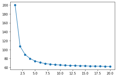
[200.0,
107.18106695239439,
88.90466866295793,
79.78035025519532,
74.3187880885867,
70.90417512718282,
68.69155318506807,
67.20013197881178,
66.15079837015878,
65.37902020765745,
64.78625525603303,
64.31246996531246,
63.9204121068791,
63.586500210988966,
63.295479267264845,
63.03724485771134,
62.80493063951664,
62.59374088047521,
62.40022787877571,
62.22183840063285]
import matplotlib as mpl
import matplotlib.pyplot as plt
import matplotlib.font_manager as fm
# 设置字体为ie黑体,以支持中文显示
font = fm.FontProperties(fname='/home/yys/.local/lib/python3.8/site-packages/matplotlib/mpl-data/fonts/ttf/msyh.ttf', size=16)
# 设置在中文字体时,能够正常显示负号(-)
mpl.rcParams['axes.unicode_minus'] = False
plt.figure(figsize=(10,10))
# 绘图预测值
plt.plot(result, "ro-", label="预测值")
# 绘制真实值
plt.plot(test_y.values, 'go--', label="真实值")
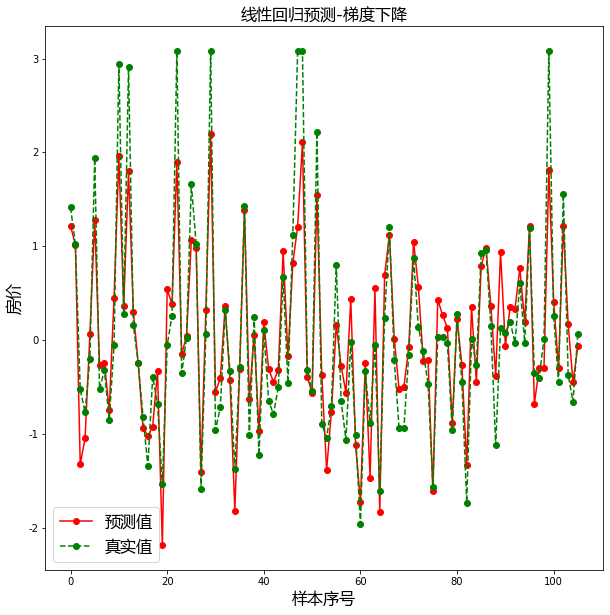
plt.title("线性回归预测-梯度下降", fontproperties=font)
plt.xlabel("样本序号", fontproperties=font)
plt.ylabel("房价", fontproperties=font)
plt.legend(prop=font, loc="best")
plt.show()
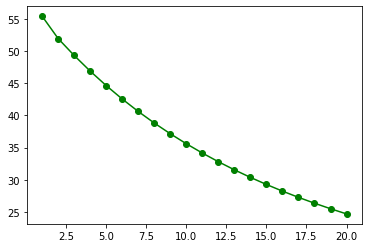
# 绘制累积误差值
plt.plot(range(1, lr.times + 1), lr.loss_, "o-")
[<matplotlib.lines.Line2D at 0x7f802e7afd30>]
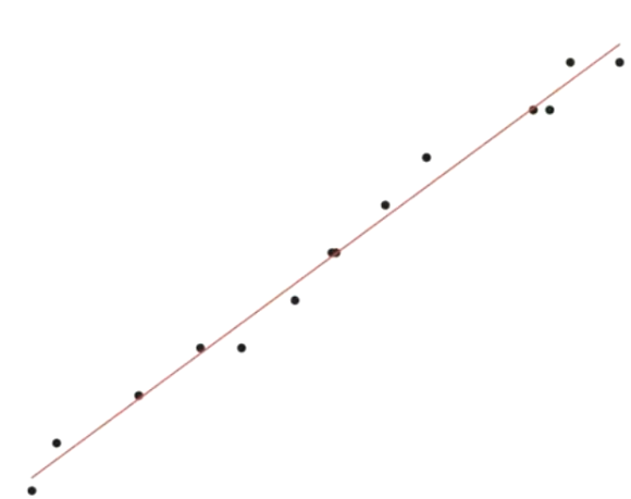
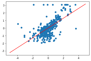
# 因为房价分析涉及多个维度,不方便可视化显示,为了方便可视化
#我们只选取其中的一个维度(rm),并画出直线,实现拟合.
lr = LinearRegression(alpha=0.0005, times=20)
t = data.sample(len(data), random_state=0)
train_X = t.iloc[:400, 5:6]
train_y = t.iloc[:400, -1]
test_X = t.iloc[400:, 5:6]
test_y = t.iloc[400:, -1]

# 对数据进行标准化处理
s = StandardScaler()
train_X = s.fit_transform(train_X)
test_X = s.transform(test_X)

s2 = StandardScaler()
train_y = s2.fit_transform(train_y)
test_y = s2.transform(test_y)

lr.fit(train_X, train_y)
result = lr.predict(test_X)
display(np.mean((result - test_y) **2))
0.46424131448205164
plt.scatter(train_X["rm"], train_y)
# 查看方程系数
display(lr.w_)
# 构建方程
# 方法1
# y = -2.6134650e-16+6.4744239e-01 * x
# plt.plot(x, y, "r")
# 方法2:
x = np.arange(-5, 5, 0.1)
plt.plot(x, lr.predict(x.reshape(-1, 1)), "r")
array([-2.6134650e-16, 6.4744239e-01])
[<matplotlib.lines.Line2D at 0x7f802e3c50d0>]
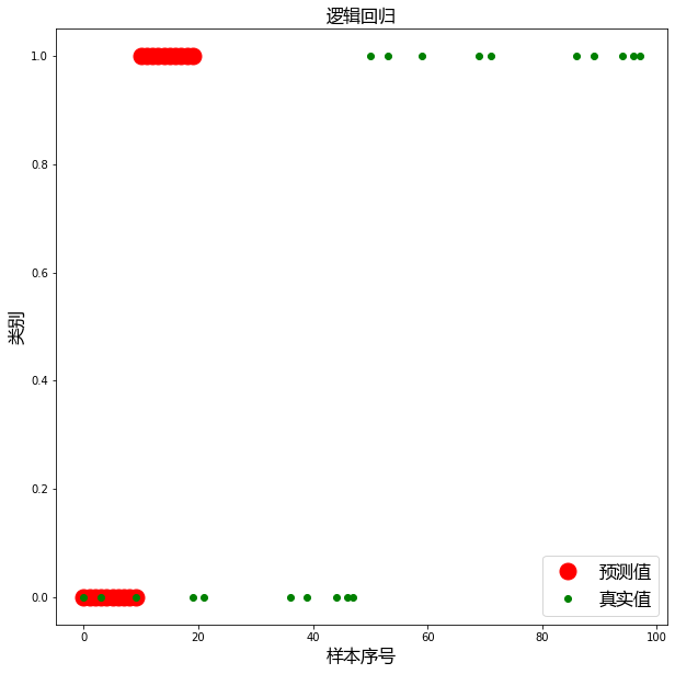
逻辑回归是一种分类模型。
\(z=W^T=W^0+W^1X^1+W^2X^2+...+W^nX^n\)
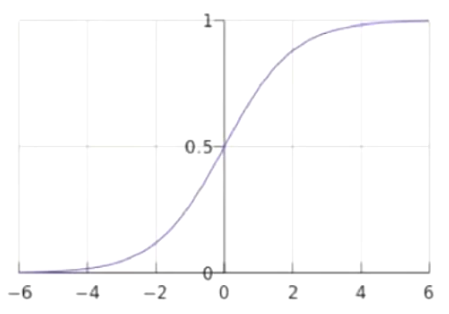
逻辑回归通过 sigmoid函数将输入值映射到[0,1]的区间范围。
\(y=p=s(z)=\frac{1}{1+e^{(-z)}}\)
逻辑回归的目标函数为:
\(J(w)=-\sum_{1}^{n}y^{(i)}log(s(z^{(i)}))+(1-y^{(i)})log(1-s(z^{(i)}))\)
因此,目标函数最小时,w的值,就是我们要求的最终权重值。
import numpy as np
import pandas as pd
data = pd.read_csv(r"./dataset/iris.csv")
# 去掉不需要的列
data.drop("Unnamed: 0", axis=1, inplace=True)
# 删除重复记录
data.drop_duplicates(inplace=True)
# data["Species"].drop_duplicates()
# setosa, versicolor, virginica
data["Species"] = data["Species"].map({"setosa":0, "versicolor": 1, "virginica": 2})
data = data[data["Species"] != 2]
class LogisticRegression:
    """使用Python语言实现逻辑回归算法."""
    def __init__(self, alpha, times):
        """初始化方法.
        Parameters
        ------
        alpha:float
        学习率
        times: int
        迭代次数.
        """
        self.alpha = alpha
        self.times = times
    def sigmoid(self, z):
        """sigmoid函数实现
        Parameters
        ------
        z:float
        自变量,值为z = w.T * x

        Return
        ----
        p:float, 值[0,1]之间.
        返回样本属于类别1的概率值,用来作为结果的预测.
        当z >= 0.5(z >= 0)时,判定为类别1, 否则判定为类别0
        """
        return 1.0 / (1.0 + np.exp(-z))
    def fit(self, X, y):
        """根据提供的训练数据,并对模型进行训.
        Parameters
        -------
        X:类数组类型.行状为:[样本数量, 特征数量]
            待训练的样本特征属性.
        y: 类数组类型.形状为:[样本数量]
            每个样本的目标值.(标签)
        """
        X = np.asarray(X)
        y = np.asarray(y)
        # 创建权重的向量,初始值为0, 长度比特征数多1.(多出来的一个是截距)
        self.w_ = np.zeros(1+X.shape[1])
        #创建损失列表,用来保存每次迭代后的损失值.
        self.loss_ = []
        for i in range(self.times):
            z = np.dot(X, self.w_[1:]) + self.w_[0]
            # 计算概率值(结果判定为之的概率值)
            p = self.sigmoid(z)
            # 根据逻辑回归的代价函数(目标函数), 计算损失值
            # 逻辑回归的代价函数(目标函数)
            # J(w) = -sum(y) * log(s(zi)) + (1-yi) * log (1-s(zi)) [i从1到n.n为样本数量]
            cost = -np.sum(y * np.log(p) + (1 - y) * np.log(1-p))
            self.loss_.append(cost)
            # 调整权重值, 根据公式,调整为: 权重(j列) = 权重(j列) + 学习率 * sum((y-s(z) * x(j)))
            self.w_[0] += self.alpha * np.sum(y - p)
            self.w_[1:] += self.alpha * np.dot(X.T, y-p)

    def predict_proba(self, X):
        """根据参数传递的样本, 对样本数据进行预测.
        Parameters
        ------
        X: 类数组类型.形状为[样本数量. 特征数量]
            待测试的样本特征(属性)
        Return
        ------
        result : 数组烈性
            预测的结果(概率值)
        """
        X = np.asarray(X)
        z = np.dot(X, self.w_[1:]) + self.w_[0]
        p = self.sigmoid(z)
        # 将预测结果变成二维数组(结构).便于后续的俄拼接
        p = p.reshape(-1, 1)
        # 将两个数组进行拼接,方向为横向拼接.
        return np.concatenate([1 - p, p], axis=1)

    def predict(self, X):
        """根据参数传递的样本,对样本数据进行预测
        ------
        X: 类数组类型.形状为[样本数量. 特征数量]
            待测试的样本特征(属性)
        Return
        ------
        result : 数组烈性
            预测的结果(分类值)
        """
        return np.argmax(self.predict_proba(X), axis=1)
t1 = data[data["Species"] == 0]
t2 = data[data["Species"] == 1]
t1 = t1.sample(len(t1), random_state=0)
t2 = t2.sample(len(t2), random_state=0)

train_X = pd.concat([t1.iloc[:40, :-1], t2.iloc[:40, :-1]], axis=0)
train_y = pd.concat([t1.iloc[:40, -1], t2.iloc[:40, -1]], axis=0)
test_X = pd.concat([t1.iloc[40:, :-1], t2.iloc[40:, :-1]], axis=0)
test_y = pd.concat([t1.iloc[40:, -1], t2.iloc[40:, -1]], axis=0)

# 鸢尾花的特征列都在同一个数量级, 我们这里可以不用进行标准化处理.
lr = LogisticRegression(alpha=0.001, times=20)
lr.fit(train_X, train_y)
# lr.predict_proba(test_X)
result = lr.predict(test_X)
# 计算准确率
# np.sum(result == test_y)
np.sum((result == test_y) / len(test_y))
1.0000000000000002
import matplotlib as mpl
import matplotlib.pyplot as plt
import matplotlib.font_manager as fm
# 设置字体为ie黑体,以支持中文显示
font = fm.FontProperties(fname='/home/yys/.local/lib/python3.8/site-packages/matplotlib/mpl-data/fonts/ttf/msyh.ttf', size=16)
# 设置在中文字体时,能够正常显示负号(-)
mpl.rcParams['axes.unicode_minus'] = False
plt.figure(figsize=(10, 10))
# 绘制预测值
plt.plot(result, "ro", ms=15, label="预测值")
# 绘制真实值
plt.plot(test_y, "go", label="预测值")
plt.title("逻辑回归", fontproperties=font)
plt.xlabel("样本序号", fontproperties=font)
plt.ylabel("类别",fontproperties=font)
plt.legend(prop=font, loc="best")
plt.show()
# 绘制目标函数的损失值
plt.plot(range(1, lr.times+1), lr.loss_, "go-")
k- means是一种最流行的聚类算法,属于无监督学习。
k- means可以在数据集分为相似的组(簇),使得组内数据的相似度较高,组间之间的相似度较低。
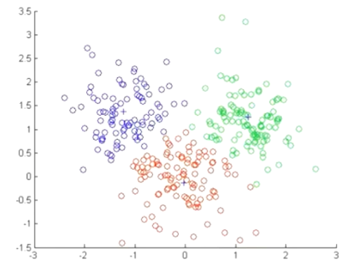
k -meann-算法的步骤如下:
- 从样本中选择k个点作为初始簇中心。
- 计算每个样本到各个簇中心的距离,将样本划分到距离最近的簇中心所对应的簇中。
- 根据每个簇中的所有样本,重新计算簇中心,并更新。
- 重复步骤2与3,直到簇中心的位置变化小于指定的阈值或者达到最大迭代次数为止。
import numpy as np
import pandas as pd
data = pd.read_csv("./dataset/order.csv")
t = data.iloc[:, -8:]
| Food% | Fresh% | Drinks% | Home% | Beauty% | Health% | Baby% | Pets% | |
|---|---|---|---|---|---|---|---|---|
| 0 | 9.46 | 87.06 | 3.48 | 0.00 | 0.00 | 0.00 | 0.0 | 0.0 |
| 1 | 15.87 | 75.80 | 6.22 | 2.12 | 0.00 | 0.00 | 0.0 | 0.0 |
| 2 | 16.88 | 56.75 | 3.37 | 16.48 | 6.53 | 0.00 | 0.0 | 0.0 |
| 3 | 28.81 | 35.99 | 11.78 | 4.62 | 2.87 | 15.92 | 0.0 | 0.0 |
| 4 | 24.13 | 60.38 | 7.78 | 7.72 | 0.00 | 0.00 | 0.0 | 0.0 |
| ... | ... | ... | ... | ... | ... | ... | ... | ... |
| 29995 | 5.80 | 0.00 | 51.30 | 0.00 | 0.00 | 0.00 | 0.0 | 42.9 |
| 29996 | 0.00 | 0.00 | 0.00 | 0.00 | 100.00 | 0.00 | 0.0 | 0.0 |
| 29997 | 9.25 | 0.00 | 77.48 | 13.27 | 0.00 | 0.00 | 0.0 | 0.0 |
| 29998 | 0.00 | 0.00 | 100.00 | 0.00 | 0.00 | 0.00 | 0.0 | 0.0 |
| 29999 | 0.00 | 0.00 | 0.00 | 0.00 | 0.00 | 0.00 | 100.0 | 0.0 |
30000 rows × 8 columns
class KMeans:
    """使用Python语言实现聚类算法"""
    def __init__(self, k, times):
        """初始化算法
        Paraters
        ------
        k:int
            聚类的个数
        time : int
            聚类的迭代次数

        """
        self. k = k
        self.times = times

    def fit(self, X):
        """根据提供的训练数据,对模型就行训练
        Parameters
        ------
        X : 类数组类型, 形状为:[样本数量,特征数量]
            待训练的样本特征属性
        """
        X = np.asarray(X)
        # 设置随机种子,以便于可以产生相同的随机序列.(随机的结果可以重现)
        np.random.seed(0)
        # 从数组中随机选择k个点作为初始聚类中心.
        self.cluster_centers_ = X[np.random.randint(0, len(X), self.k)]
        self.labels_ = np.zeros(len(X))

        for t in range(self.times):
            for index, x in enumerate(X):
                # 计算每个样本与聚类的中心距离
                dis = np.sqrt(np.sum((x - self.cluster_centers_) **2 , axis=1))
                # 将最小距离的索引赋值给标签数组,索引的值就是当前所属的簇.范围为[0, k - 1]
                self.labels_[index] = dis.argmin()
            # 循环遍历每一个簇
            for i in range(self.k):
                # 计算每个簇内所有的均值,更新聚类中心
                self.cluster_centers_[i] = np.mean(X[self.labels_ == i], axis=0)

    def predict(self, X):
        """根据参数传递的样本, 对样本数据进行预测.(预测样本属于哪一个簇中)
        Parameters
        ------
        X:类数组类型,形状为:[样本数量, 特征数量]
        Return
        ------
        result:数组类型
            预测结果,每一个X所属的簇
        """
        X = np.asarray(X)
        result = np.zeros(len(X))
        for index, x in enumerate(X):
            # 计算样本每个聚类中心的距离
            dis = np.sqrt(np.sum((x - self.cluster_centers_) ** 2, axis=1))
            # 找距离最近的聚类中心,划分类别
            result[index] = dis.argmin()
        return result
kmeans = KMeans(3, 50)
kmeans.fit(t)
kmeans.cluster_centers_
array([[46.33977936,  8.93380516, 23.19047005, 13.11741633,  4.8107557 ,
         1.17283735,  1.35704647,  0.95392773],
       [19.5308009 , 50.42856608, 14.70652695,  7.89437019,  3.69829234,
         0.91000428,  1.92515077,  0.82113238],
       [ 7.93541008,  4.56182052, 30.65583437, 18.57726789,  8.61597195,
         1.28482514, 26.81950293,  1.30158264]])
#查看某个簇内所有样本数据
t[kmeans.labels_ == 0]
| Food% | Fresh% | Drinks% | Home% | Beauty% | Health% | Baby% | Pets% | |
|---|---|---|---|---|---|---|---|---|
| 15 | 48.23 | 20.37 | 15.38 | 8.29 | 7.73 | 0.0 | 0.0 | 0.0 |
| 23 | 24.10 | 22.29 | 38.69 | 14.92 | 0.00 | 0.0 | 0.0 | 0.0 |
| 24 | 36.51 | 31.93 | 27.18 | 4.38 | 0.00 | 0.0 | 0.0 | 0.0 |
| 40 | 22.76 | 0.00 | 0.00 | 77.24 | 0.00 | 0.0 | 0.0 | 0.0 |
| 43 | 65.64 | 12.36 | 21.99 | 0.00 | 0.00 | 0.0 | 0.0 | 0.0 |
| ... | ... | ... | ... | ... | ... | ... | ... | ... |
| 29974 | 33.93 | 0.00 | 17.46 | 41.46 | 7.15 | 0.0 | 0.0 | 0.0 |
| 29977 | 45.10 | 0.00 | 26.68 | 28.22 | 0.00 | 0.0 | 0.0 | 0.0 |
| 29988 | 28.21 | 0.00 | 48.34 | 23.44 | 0.00 | 0.0 | 0.0 | 0.0 |
| 29989 | 61.32 | 0.00 | 23.34 | 15.34 | 0.00 | 0.0 | 0.0 | 0.0 |
| 29990 | 29.74 | 28.72 | 19.52 | 22.02 | 0.00 | 0.0 | 0.0 | 0.0 |
9382 rows × 8 columns
kmeans.predict([[30, 30, 40,0, 0, 0, 0, 0], [0, 0, 0, 0, 0, 30, 30, 40], [30,30, 0, 0, 0, 0, 20, 20]])
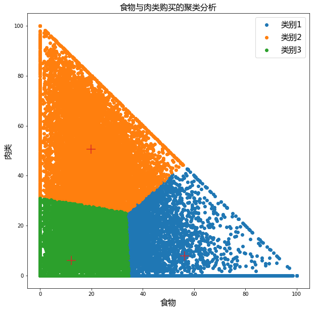
t2 = data.loc[:,"Food%":"Fresh%"] # 选择两项进行可视化展示
kmeans = KMeans(3, 50)
kmeans.fit(t2)
import matplotlib as mpl
import matplotlib.pyplot as plt
import matplotlib.font_manager as fm
# 设置字体为ie黑体,以支持中文显示
font = fm.FontProperties(fname='/home/yys/.local/lib/python3.8/site-packages/matplotlib/mpl-data/fonts/ttf/msyh.ttf', size=16)
# 设置在中文字体时,能够正常显示负号(-)
mpl.rcParams['axes.unicode_minus'] = False
plt.figure(figsize=(10, 10))
plt.scatter(t2[kmeans.labels_ == 0].iloc[:, 0], t2[kmeans.labels_ == 0].iloc[:, 1], label="类别1")
plt.scatter(t2[kmeans.labels_ == 1].iloc[:, 0], t2[kmeans.labels_ == 1].iloc[:, 1], label="类别2")
plt.scatter(t2[kmeans.labels_ == 2].iloc[:, 0], t2[kmeans.labels_ == 2].iloc[:, 1], label="类别3")
# 绘制聚类中心
plt.scatter(kmeans.cluster_centers_[:, 0], kmeans.cluster_centers_[:, 1], marker="+", s=300)

plt.title("食物与肉类购买的聚类分析", fontproperties=font)
plt.xlabel("食物", fontproperties=font)
plt.ylabel("肉类", fontproperties=font)
plt.legend(prop=font, loc="best")
plt.show()
Python中TypeError: 'str' object is not callable解决方法
plt.title("食物与肉类购买的聚类分析", fontproperties=font)
解决方案:重启服务

具体的原因:1.之前的不正确输入,如:plt.xlabel=‘time’ or plt.xlabel 的各种不正确赋值。
并且 ,* xlabel* , 有明确 的不可改性。所以:即使您在最后改回正确的,也任然报错。
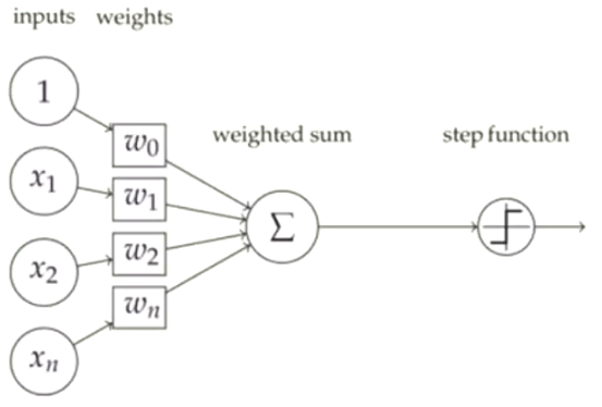
感知器是一种人工神经网络,其模拟生物上的神经元结构。

感知器是一个二分类器,其将净输入为
\(z = W^TX=W^0+W^1X^1+W^2X^2+...+W^nX^n\)
通过激活函数q(z),就可以将其映射为1或-1
\(\varphi(z)= \begin{cases} 1, z \ge\theta \\ -1, z<\theta \end{cases}\)
import numpy as np
import pandas as pd
data = pd.read_csv(r"./dataset/iris.csv")
data.drop("Unnamed: 0", axis=1, inplace=True)
data.drop_duplicates(inplace=True)
# 之所以映射成1与-1,而不是之前的0,1,2是因为感知器预测结果为之与-1
# 目的是为了与感知器预测的结果相符
data["Species"] = data["Species"].map({"setosa":0, "versicolor": 1, "virginica": -1})
# data["Species"].value_counts()  #统计"Species"的类别
data = data[data["Species"] != 0]
# data
| Sepal.Length | Sepal.Width | Petal.Length | Petal.Width | Species | |
|---|---|---|---|---|---|
| 50 | 7.0 | 3.2 | 4.7 | 1.4 | 1 |
| 51 | 6.4 | 3.2 | 4.5 | 1.5 | 1 |
| 52 | 6.9 | 3.1 | 4.9 | 1.5 | 1 |
| 53 | 5.5 | 2.3 | 4.0 | 1.3 | 1 |
| 54 | 6.5 | 2.8 | 4.6 | 1.5 | 1 |
| ... | ... | ... | ... | ... | ... |
| 145 | 6.7 | 3.0 | 5.2 | 2.3 | -1 |
| 146 | 6.3 | 2.5 | 5.0 | 1.9 | -1 |
| 147 | 6.5 | 3.0 | 5.2 | 2.0 | -1 |
| 148 | 6.2 | 3.4 | 5.4 | 2.3 | -1 |
| 149 | 5.9 | 3.0 | 5.1 | 1.8 | -1 |
99 rows × 5 columns
class Perceptron:
    """使用Python语言实现感知器算法,实现二分类"""
    def __init__(self, alpha, times):
        """初始化方法
        Parameters
        -----
        alpha : fload
            学习率
        tines: int
        最大迭代次数
        """
        self.alpha = alpha
        self.times = times

    def step(self, z):
        """阶跃函数.
        Parameters
        ------
        z: 数组类型(或者标量类型)
            阶越函数的参数,可以根据z的值,返回1或-1(这样可以实现二分类)
        Returns
        -------
        value : int
            如果 z >= 0, 返回1, 否则返回-1
        """
        return np.where(z >= 0, 1, -1) # Z可以数组形式

    def fit(self, X, y):
        """根据提供的训练数据,对模型进行训练
        Parameters
        ------
        X : 类数组类型.形状:[样本数量, 特征数量]
            待训练的样本数据
        y : 类数组类型.形状: [样本数量]
            每个样本的目标值.(分类)
        """
        X = np.asarray(X)
        y = np.asarray(y)
        # 创建权重的向量,初始值为0,长度比特征多1.(多出的一个就是截距)
        self.w_ = np.zeros(1 + X.shape[1])
        # 创建损失值列表,用来保存每次迭代后的损失值
        self.loss_ = []
        # 循环制定的次数.
        for i in range(self.times):
            # 感知与逻辑回归的区别,逻辑回归中,使用所有的样本梯度,然后进行更新权重.
            # 而感知器中,是使用单个样本,依次进行计算梯度,更新权重.
            loss = 0
            for x, target in zip(X, y):
                # 计算预测值
                y_hat = self.step(np.dot(x, self.w_[1:]) + self.w_[0])
                loss += y_hat != target
                # 更新权重.

                #更新公式: w(j) = w(j) + 学习率 * (真实值-预测值) * x (j)
                self.w_[0] += self.alpha * (target - y_hat)
                self.w_[1:] += self.alpha * (target - y_hat) * x
            # 将循环中累计的误差值加到误差列表中
            self.loss_.append(loss)

    def predict(self, X):
        """根据参数传递的样本,对样本数据进行预测.(1或-1)
        Parameters
        -------
        X:类数组类型, 形状为:[样本数量, 特征数量]
            待预测的样本特征
        Returns
        ------
        result :数组类型
            预测的结果值(分类1或-1)
        """
        return self.step(np.dot(X, self.w_[1:]) + self.w_[0])
t1 = data[data["Species"] == 1]
t2 = data[data["Species"] == -1]
t1 = t1.sample(len(t1), random_state=0)
t2 = t2.sample(len(t2), random_state=0)
train_X = pd.concat([t1.iloc[:40, :-1], t2.iloc[:40, :-1]], axis=0)
train_y = pd.concat([t1.iloc[:40, -1], t2.iloc[:40, -1]], axis=0)
test_X = pd.concat([t1.iloc[40:, :-1], t2.iloc[40:, :-1]], axis=0)
test_y = pd.concat([t1.iloc[40:, -1], t2.iloc[40:, -1]], axis=0)
p = Perceptron(0.1, 10)
p.fit(train_X, train_y)
result = p.predict(test_X)
display(result)
display(test_y.values)
display(p.w_)
display(p.loss_)
[1, 3, 2, 2, 2, 3, 2, 2, 2, 2]
import matplotlib as mpl
import matplotlib.pyplot as plt
import matplotlib.font_manager as fm
# 设置字体为ie黑体,以支持中文显示
font = fm.FontProperties(fname='/home/yys/.local/lib/python3.8/site-packages/matplotlib/mpl-data/fonts/ttf/msyh.ttf', size=16)
# 设置在中文字体时,能够正常显示负号(-)
mpl.rcParams['axes.unicode_minus'] = False
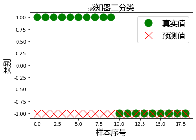
# 绘制真实值
plt.plot(test_y.values, "go", ms=15, label="真实值")
# 绘制预测值
plt.plot(result, "rx", ms=15, label="预测值")
plt.title("感知器二分类", fontproperties=font)
plt.xlabel("样本序号", fontproperties=font)
plt.ylabel("类别", fontproperties=font)
plt.legend(prop=font, loc="best")
plt.show()
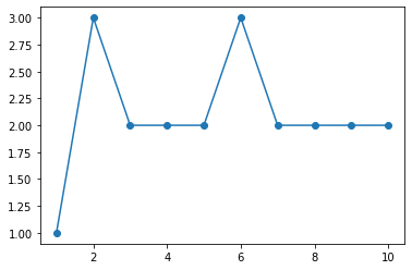
#绘制目标函数的损失值
plt.plot(range(1, p.times+1), p.loss_, "o-")
本文作者: 永生
本文链接: https://yys.zone/detail/?id=180
版权声明: 本博客所有文章除特别声明外,均采用 CC BY-NC-SA 4.0 许可协议。转载请注明出处!
评论列表 (0 条评论)